Snappy looking calcium imaging videos

Want to make your calcium imaging videos look better for presentations? Read on. Or just skip to the recipe section below. First, I’ll discuss the motivation a bit.

One of my refrains when I talk about making slides for scientific presentations is: “Never tell your audience, ‘this is hard to see, but it looks okay on my laptop’.” We’ve all heard some version of that many times. It’s natural and understandable, but it’s also avoidable. Show respect to your audience by preparing in advance.

Unless you’re giving a talk on something excellent like an 8k high dynamic range OLED monitor, all of your slides are definitely going to look poor compared to your laptop display. Very low contrast. Count on it. Expect it. Plan for it.

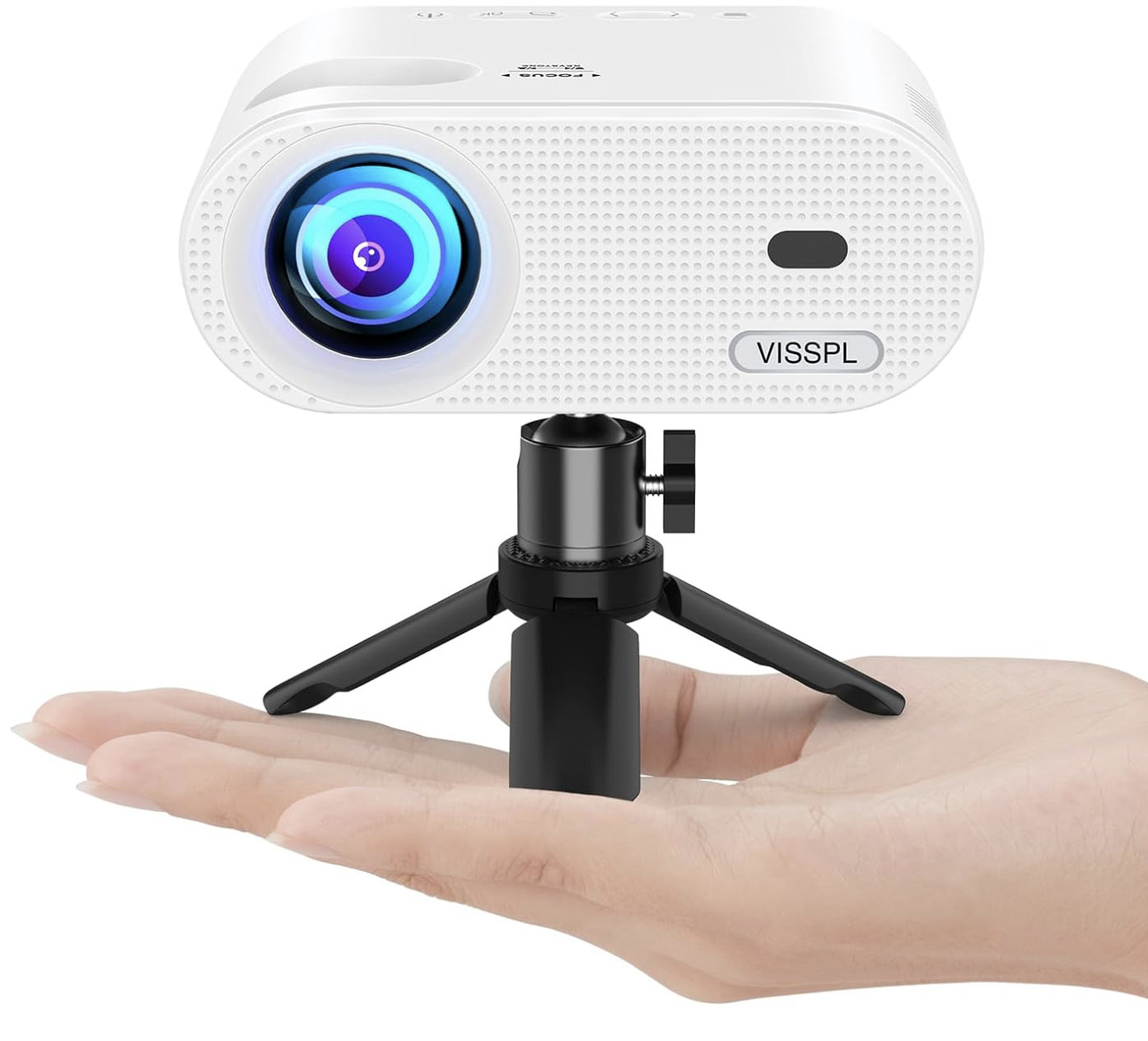
All of your images need to have very high contrast. Test them out on the worst projector you can find. Like a cheap VGA mini projector you buy on the internet for fifty bucks. Make sure that they look good on that. THEN go give your talk.

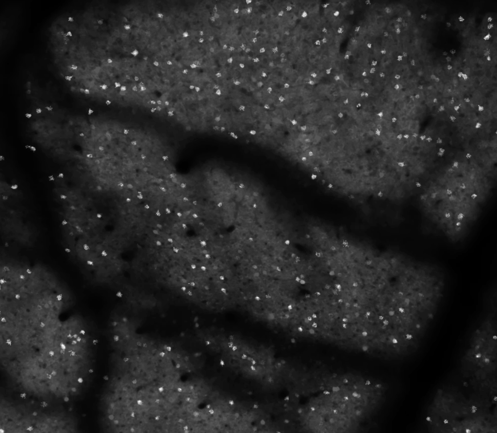
I show a lot of two-photon calcium imaging videos in my talks. It’s a big part of how I study neural circuitry. These videos are beautiful to me. Perception and behavior, all of our experiences and interactions with the world, are built from countless tiny millisecond-long millivolt-level excursions. These vast conversations, spanning the entire brain every second, are an insanely beautiful choreography. And large field-of-view two-photon calcium imaging distills this computational choreography into visible light.

The type of calcium imaging I do prioritizes the field-of-view and temporal resolution. I want as many neurons as I can sample, at around 10 frames per second, with each neuron having enough samples to provide a high fidelity measurement of the fluorescence dynamics of a calcium indicator. The spatial sampling is typically well below the Nyquist criterion, because I don’t care about the shape of cells. I just need enough pixels per neuron to get a high fidelity signal (often this is 10-20 pixels). We are often operating in the regime where shot noise is a visible factor, making due with as few photons per pixel as we can, so that we can distribute them broadly in space and time, and obtain sufficient temporal resolution for as many neurons as possible.

So the individual frames can be a bit ugly. That’s okay. They are a bit noisy. We’re averaging over all of the pixels for individual cells before we do our analysis. The individual frames can look pretty rough, and we still get high fidelity measurements of indicator dynamics from them. So while the aficionados can see the beauty in raw calcium imaging videos, a general audience might be less impressed. They might wonder what we’re so excited about. It can be helpful to process the videos to give a better impression of the data.

Sometimes simply adjusting the look-up-table parameters (min and max values, and gamma) can help a lot. Perhaps a snappy color look-up-table can help. I typically prefer to stick with black-and-white for this type of data. Colored look up tables can lead to unpredictable results with color reproduction on projectors, low contrast, and/or colorblind audience members. Black-and-white is a bit more general purpose, and can be sufficient in many cases.

Recipe

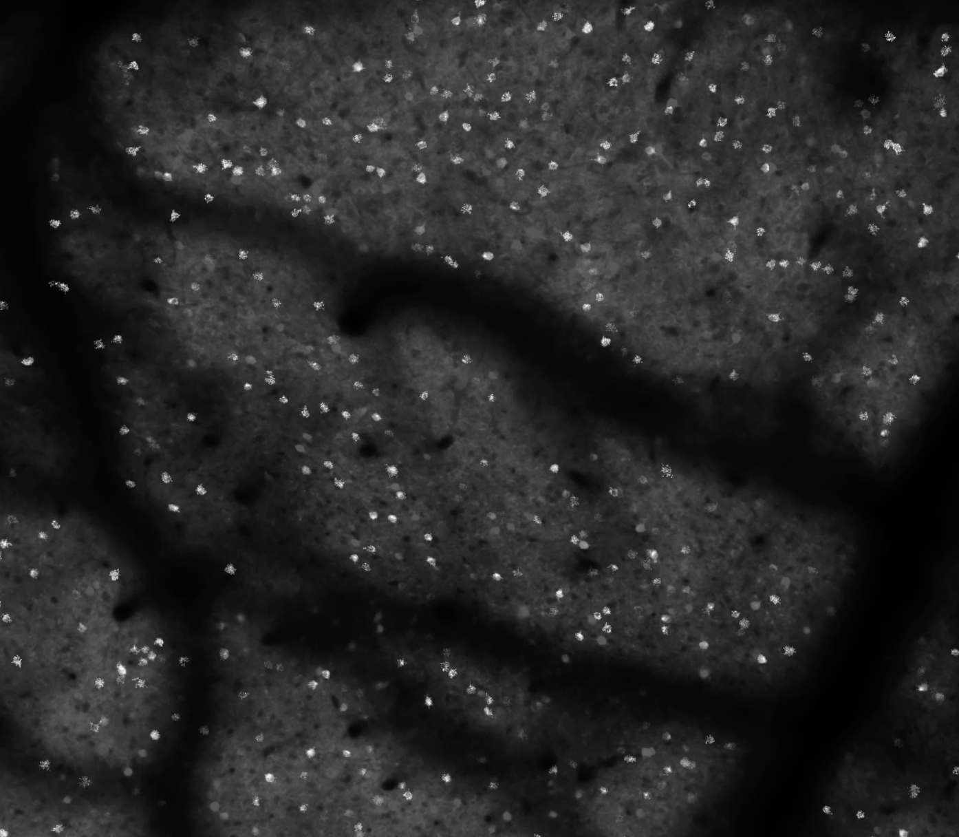
Let’s think about this problem another way. Like I said above, the individual frames can be sort of ugly and that’s okay because we average signals over the pixels assigned to individual cells. This leads to high fidelity signals that we use for analysis. Instead of asking the audience to have the eyes of an aficionado and recognize the quality of the raw data, let’s go ahead and do the analysis and then map that back into the video.

First, let’s analyze the data. Apply motion correction, segment the image, extract the raw traces, do the neuropil subtraction, and infer spikes. Hold on to that for a moment.

Second, let’s take a projection of the video stack. Either a max, average, or std dev projection. Whatever looks good. Sometimes it’s better to run the projection on a subsection of the stack, not the full stack.

Third, let’s work backwards. Take the inferred spike trains and convolve them with a calcium indicator kernel (near-instantaneous onset and an exponential decay). Then use those convolved signals to modulate the brightness of the ROIs mapped back onto the projected image.

Filip Tomaska worked on this idea and wrote the code to work things out. At first, we used binary ROI masks, and that was okay, but looked a bit crude and pixelated. Using a max projection of the ROI gave us some shading that looked a bit more pleasing. Another thing we did is make the projection a bit dim, so that bright cells can pop out better when they increase in brightness over time.

Last of all, we adjusted the function for mapping the signal trace to ROI brightness. A straight linear mapping is a problem because single spike signals are hard to see by eye, and the bursts are relatively rare. So it gives the impression that there is less activity than we can actually detect. Projectors and displays often only have 8 bits of dynamic range for brightness and can be effectively worse depending on ambient lighting. The actual signals we use for analysis can have 12+ bits of dynamic range. So for display I wanted a function that would be linear at low values, to make single spikes visible, and then quickly saturate at high values. The hyperbolic tangent (tanh) function worked well for that. Here’s the end result:

And here’s the code by Filip Tomaska (below). We use Suite2p and MCMC for spike inference. This code takes in a mean image, stat, and iscell from Suite2p + spiketimes from MCMC.

function overlayBlinkingROIs_onMean(meanIm, out, stat, iscellFlags, varargin)
% Overlay blinking ROIs (alpha ~ convolved spikes) on a mean projection.
%
% Inputs
%   meanIm        : [Ly x Lx] mean projection (double/single/uint)
%   out.path1_phys.spiketimes :
%                    - cell array: {k} seconds
%                    - struct array: (k).spks seconds  (your case)
%                    Count must equal sum(iscellFlags(:,1)==1)
%   stat          : Suite2p ROI struct(s): stat{1,i}.xpix/ypix or stat(i)
%   iscellFlags   : [Nroi x 2], first col 1 = cell, 0 = not cell
%
% Name/Value options
%   'Params'       : struct('tau_rise',0.07,'tau_decay',0.7)  (default)
%   'FPS'          : native fps of original acquisition (default 15)
%   'DurationSec'  : total duration to render (default: from last spike + margin)
%   'NFrames'      : override number of frames (else computed from DurationSec)
%   'Output'       : output MP4 filename (default 'roi_on_mean_2x.mp4')
%   'BaseContrast' : [low high] percentiles for base image (default [1 99])
%   'ClipPercent'  : soft-clip traces percentile (default 99)
%   'GlobalScale'  : normalize traces by global max (default true)
%   'OverlayColor' : [R G B] single color (default [0 1 0])
%   'ColorByROI'   : true = distinct colors per ROI (default false)
%   'AlphaMax'     : max overlay alpha (default 0.85)
%
% Example
%   params = struct('tau_rise',0.07,'tau_decay',0.7);
%   overlayBlinkingROIs_onMean(mean(M1,3), out, stat, iscell, ...
%       'Params', params, 'FPS', 15, 'Output','blink_on_mean.mp4');

%^by chatGPT for better dissemination

%  parse options
p = inputParser;
p.addParameter('Params', struct('tau_rise',0.07,'tau_decay',0.7));
p.addParameter('FPS', 15);
p.addParameter('DurationSec', []);
p.addParameter('NFrames', []);
p.addParameter('Output', 'roi_on_mean_2x.mp4', @ischar);
p.addParameter('BaseContrast', [1 99], @(v)isnumeric(v)&&numel(v)==2);
p.addParameter('ClipPercent', 99, @(x)isnumeric(x)&&isscalar(x)&&x>0&&x<=100);
p.addParameter('GlobalScale', true, @islogical);
p.addParameter('OverlayColor', [0 1 0], @(v)isnumeric(v)&&numel(v)==3);
p.addParameter('ColorByROI', false, @islogical);
p.addParameter('AlphaMax', 0.85, @(x)isnumeric(x)&&isscalar(x)&&x>=0&&x<=1);
p.parse(varargin{:});
opt = p.Results;

% kernel params (support params.'6s' style too)
params = opt.Params;
if isfield(params,'tau_rise') && isfield(params,'tau_decay')
    tau_rise  = params.tau_rise;  tau_decay = params.tau_decay;
elseif isfield(params,'6s')
    tau_rise  = params.('6s').tau_rise;  tau_decay = params.('6s').tau_decay;
else
    error('Params must have tau_rise/tau_decay or a key like params.''6s''.');
end
fps_native = opt.FPS;

% ?? select ROIs (only iscell==1) and grab spikes container ?????????????????
roiIsCell = find(iscellFlags(:,1)==1);
nKeep     = numel(roiIsCell);

if ~isfield(out,'path1_phys') || ~isfield(out.path1_phys,'spiketimes')
    error('out.path1_phys.spiketimes not found.');
end
spkBag = out.path1_phys.spiketimes; % may be cell array or struct array
isSpkCell   = builtin('iscell', spkBag);
isSpkStruct = isstruct(spkBag);
if numel(spkBag) ~= nKeep
    error('spiketimes count (%d) != number of iscell==1 (%d).', numel(spkBag), nKeep);
end

% helper for spike times (seconds) per kept index k
get_spikes = @(k) local_get_spikes(spkBag, k, isSpkCell, isSpkStruct);

% get image size, roi etc...
[Ly,Lx,zeroBased] = local_infer_image_size(stat, iscellFlags);
maskIdx = cell(nKeep,1);
for k = 1:nKeep
    roi = roiIsCell(k);
    S = local_stat_at(stat, roi);
    y = S.ypix(:); x = S.xpix(:);
    if zeroBased, y = y+1; x = x+1; end
    y = max(1, min(Ly, round(y)));
    x = max(1, min(Lx, round(x)));
    maskIdx{k} = sub2ind([Ly Lx], y, x);
end

% process mean projection
% 
meanIm = im2double(imresize(meanIm, [Ly Lx]));
lo = prctile(meanIm(:), opt.BaseContrast(1));
hi = prctile(meanIm(:), opt.BaseContrast(2));
baseIm = (meanIm - lo) / max(hi - lo, eps);
baseIm = min(max(baseIm,0),1);

% infer timeline from last spike time
if ~isempty(opt.NFrames)
    nFrames = opt.NFrames;
else
    if ~isempty(opt.DurationSec)
        Tsec = opt.DurationSec;
    else
        lastSpike = 0;
        for k = 1:nKeep
            st = get_spikes(k);
            if ~isempty(st), lastSpike = max(lastSpike, max(st)); end
        end
        Tsec = lastSpike + 5*max(tau_decay,tau_rise); % tail margin
        if ~isfinite(Tsec) || Tsec<=0, Tsec = 10; end % fallback 10s
    end
    nFrames = max(1, round(Tsec * fps_native));
end
dt = 1 / fps_native;
t_edges = 0:dt:(nFrames*dt);

% GECI kernel
tmax = 5*max(tau_decay, tau_rise);
kt   = 0:dt:tmax;
kern = exp(-kt./tau_decay) - exp(-kt./tau_rise);
kern = max(kern, 0);
if max(kern)>0, kern = kern./max(kern); else, warning('Kernel is zero.'); end

% convolve spikes to Ca
traces = zeros(nKeep, nFrames, 'single');
globalMax = 0;
for k = 1:nKeep
    st = get_spikes(k);
    if isempty(st), continue; end
    bcounts     = histcounts(st, t_edges);          % length nFrames
    convsig     = conv(single(bcounts), single(kern), 'same');
    traces(k,:) = convsig;
    if opt.GlobalScale, globalMax = max(globalMax, max(convsig)); end
end
if opt.GlobalScale
    traces = traces / max(eps, globalMax);
else
    for k = 1:nKeep
        m = max(traces(k,:)); if m>0, traces(k,:) = traces(k,:)/m; end
    end
end
traces = min(max(traces,0),1);
if opt.ClipPercent < 100
    v = traces(:); v = v(v>0);
    if ~isempty(v)
        vmax = prctile(v, opt.ClipPercent);
        if isfinite(vmax) && vmax>0, traces = min(traces / vmax, 1); end
    end
end

% overlay color def
if opt.ColorByROI
    cmap = hsv(nKeep);
else
    cmap = repmat(opt.OverlayColor(:).', nKeep, 1);
end

% write as mp4 because boss hates avi.
playback_coeff = 2: % how many times faster is the playback
fps_out = playback_coeff * fps_native;
vw = VideoWriter(opt.Output, 'MPEG-4'); vw.FrameRate = fps_out; vw.Quality = 95; open(vw);
fprintf('Writing %s (%dx%d), %d frames @ %.1f fps (2×)...\n', opt.Output, Lx, Ly, nFrames, fps_out);

for f = 1:nFrames
    % start with static base
    frameRGB = repmat(baseIm, [1 1 3]);
    % alpha-blend each ROI using trace as alpha driver
    for k = 1:nKeep
        a = min(1, opt.AlphaMax * double(traces(k,f)));
        if a<=0, continue; end
        idx = maskIdx{k};
        for c = 1:3
            col = cmap(k,c);
            tmp = frameRGB(:,:,c);
            tmp(idx) = (1 - a).*tmp(idx) + a.*col;
            frameRGB(:,:,c) = tmp;
        end
    end
    writeVideo(vw, im2uint8(frameRGB));
end
close(vw);
fprintf('Done.\n');

end

%helpers
function S = local_stat_at(stat, ii)
    if builtin('iscell', stat), S = stat{1,ii}; else, S = stat(ii); end
end

function [Ly,Lx,zeroBased] = local_infer_image_size(stat, iscellFlags)
    nROIs = size(iscellFlags,1);
    allY = []; allX = [];
    for ii = 1:nROIs
        S = [];
        if builtin('iscell', stat)
            if ii<=numel(stat) && ~isempty(stat{1,ii}), S = stat{1,ii}; end
        else
            if ii<=numel(stat) && ~isempty(stat(ii)),   S = stat(ii);    end
        end
        if ~isempty(S) && isfield(S,'ypix') && isfield(S,'xpix') ...
                       && ~isempty(S.ypix) && ~isempty(S.xpix)
            allY = [allY; S.ypix(:)];
            allX = [allX; S.xpix(:)];
        end
    end
    if isempty(allY) || isempty(allX)
        error('Could not infer image size: stat entries missing ypix/xpix.');
    end
    zeroBased = (min(allY) == 0) || (min(allX) == 0);
    Ly = max(allY) + double(zeroBased);
    Lx = max(allX) + double(zeroBased);
end

function st = local_get_spikes(spkBag, k, isSpkCell, isSpkStruct)
    if isSpkCell
        st = spkBag{k};
    elseif isSpkStruct
        if isfield(spkBag, 'spks')
            st = spkBag(k).spks;
        else
            cand = {'t','times','spike_times','spikeTimes'};
            got = [];
            for ii=1:numel(cand)
                if isfield(spkBag, cand{ii}), got = spkBag(k).(cand{ii}); break; end
            end
            if isempty(got), error('spiketimes struct lacks .spks (or known aliases).'); end
            st = got;
        end
    else
        error('out.path1_phys.spiketimes must be cell or struct array.');
    end
    if isempty(st), st = []; else, st = st(:)'; end
end