Tons of 2p spectra – twophotondyes.com
Posted in Tips
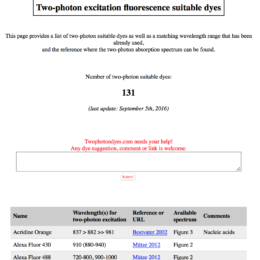
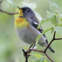
Daniel Fiole is curating a nice resource for 2p cross sections: twophotondyes.com
There’s a lot here. It’s not just dyes, he has links for fluorescent proteins as well, and there’s 3p…
Daniel Fiole is curating a nice resource for 2p cross sections: twophotondyes.com
There’s a lot here. It’s not just dyes, he has links for fluorescent proteins as well, and there’s 3p…
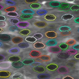
Collaborative Approach for eNhanced Denoising under Low-light Excitation, or CANDLE, is a denoising algorithm specialized for the type of images that are acquired in 2-photon imaging applications. There’s code for both ImageJ and MATLAB…
George McNamara recently posted a comment on spectra, which referenced this online app which is handy.
…
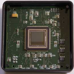
UNC-Chapel Hill’s Computer Integrated Systems for Microscopy and Manipulation team released a new version of their popular ImageSurfer software. All 64-bit, with versions for Linux, OSX, and Windows.
…
Parula is the new default colormap for MATLAB (namesake above, actual map below). It probably collapses to grey better than jet (which is good for colorblind readers).
You aficionados care dearly about…
(This post by the SIMA Team.)
The SIMA (Sequential IMage Analysis) package facilitates analysis of time-series imaging data arising from fluorescence microscopy. The functionality of this package includes:
– correction of motion artifacts
– segmentation of imaging…
About 25 years ago, pro-level audio recording technology was prohibitively expensive for home studios. Then, digital audio technology like the Alesis ADAT enabled working class musicians to produce high fidelity recordings. The…
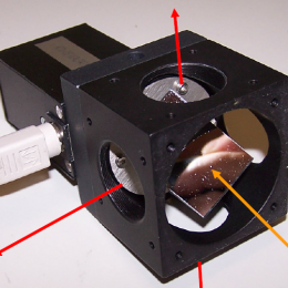
Vojnovic’s group at Oxford has dozens of technical notes. Most are concise, and include software code, if applicable. SolidWorks files and PCB files are available on request.
Here are a few examples:
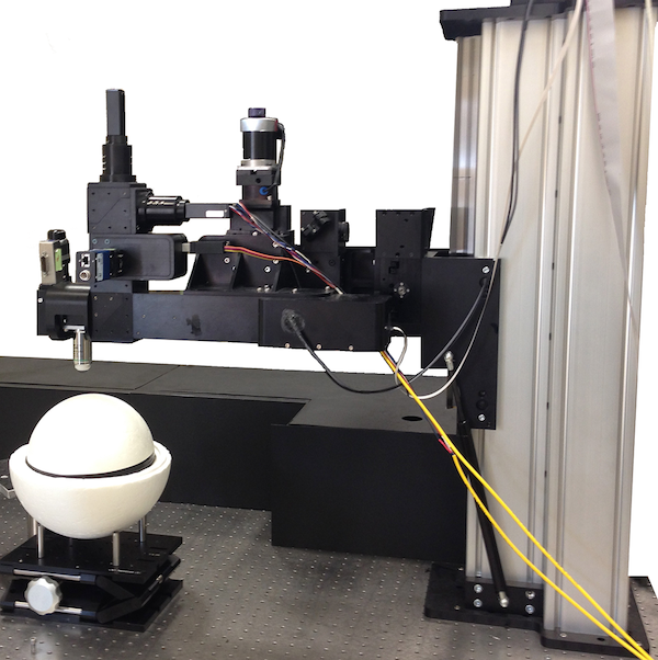
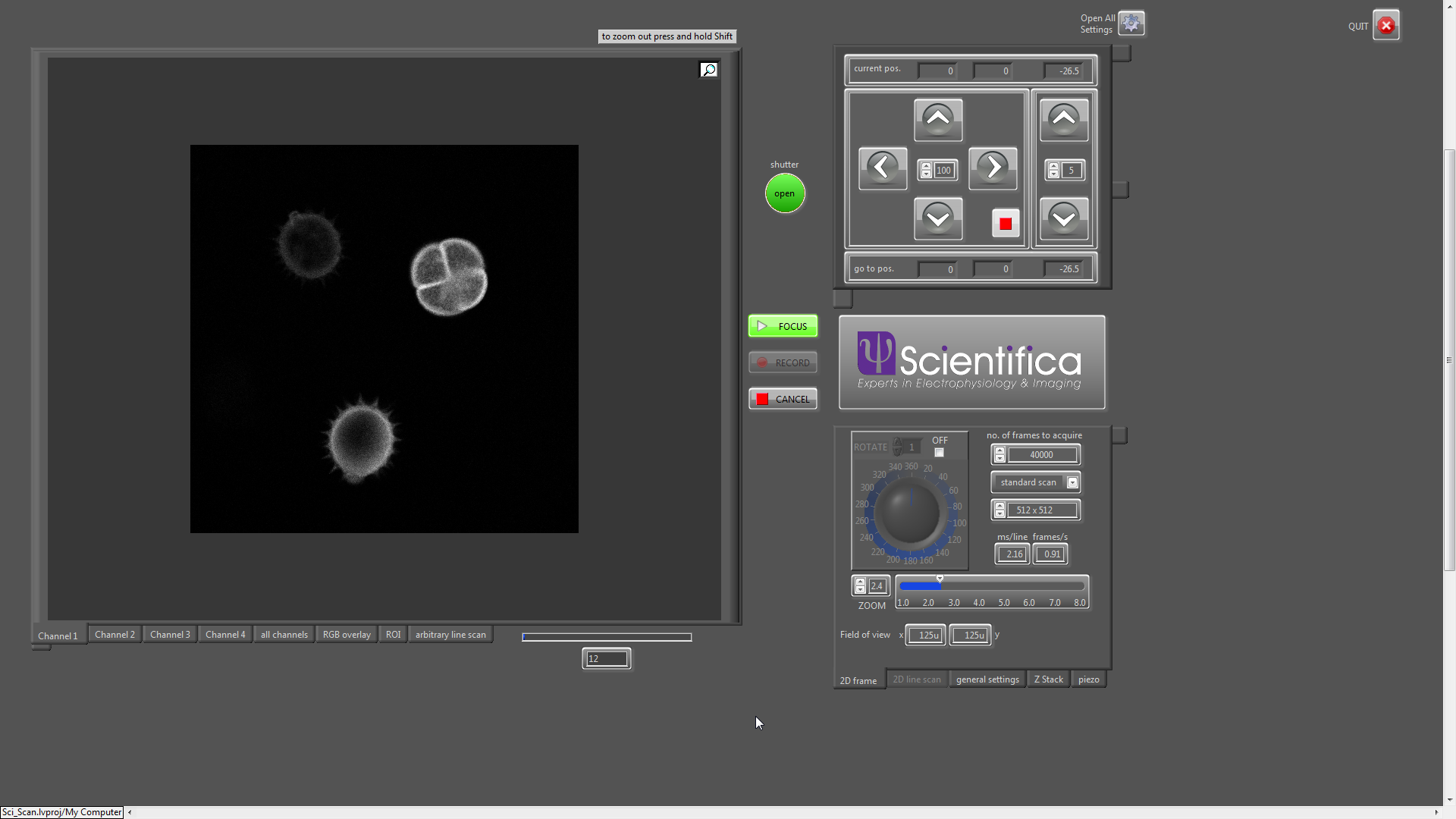
My friend Bruno has written some very nice software for Scientifica’s two photon microscope systems. It’s called SciScan.
It’s written in LabVIEW and runs both their conventional galvo and resonant…
Here’s an update on the scope from Joshua Trachtenberg’s team. If you want one, contact them at: info.neurolabware@gmail.com
This is another moving objective microscope, like the Sutter (Denk/MOM) scope, and the Thorlabs scope. Here’s…
Post by Jeffrey Stirman
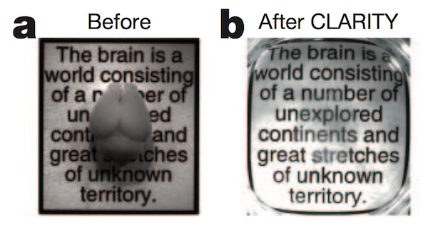
The opacity of the brain is one barrier to optically imaging individual neurons and their connections. Scattering in tissue is the main reason tissue is not transparent; absorption also plays a…
Post by Christian Wilms
I’ll admit it: I’m lazy. When I use a calcium indicator and need to know its physico-chemical properties, I like to simply look it up in the manufacturer’s catalogue or…
Many red fluorescent proteins go through a green fluorescent stage prior to becoming fully folded into their mature red fluorescent state. In fact, some proteins can be photoswitched in and/or out of their mature…
Last Monday, Labrigger covered HelioScan, a LabVIEW-based, two-photon laser scanning microscopy software suite.
Marcel van ‘t…