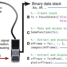
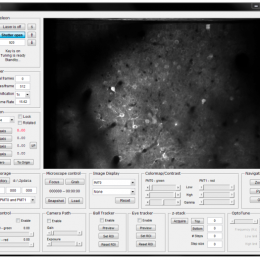
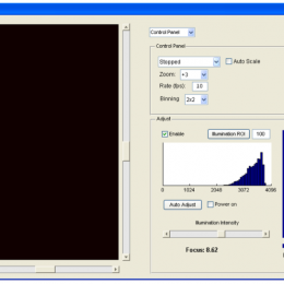
Posts tagged with MATLAB

hg2

Undocumented MATLAB has an in depth look at the next generation graphics handler for MATLAB which you can use today, although it’s not officially released yet. Use the command line option “-hgVersion 2″ when launching MATLAB. See the post for more details.

tpp

s1

More open source software to check out.

Two-Photon Processor and SeNeCA – A freely available software package to process data from two-photon calcium imaging at speeds down to several ms per frame.
Jakub Tomek, Ondrej Novak, and Josef Syka
TJ Neurophysiol published 10 April 2013, 10.1152/jn.00087.2013

It’s notable in that it is an “all-in-one” package that’s freely available.

The image processing to detect cells and draw ROIs seems to work pretty good, even with poor S:N. I’d like to see it operate on GCaMP images, since those are more challenging in some ways. Cells labeled with Oregon Green BAPTA-1 tend to exhibit spherical patterns of somatic fluorescence, but GCaMP, when it’s working well, does not brightly label the nucleus, so the shape of the ideal ROI is quite different. Plus, it’s nice to pick up dendrites and other features, not just somata.

See also, Vogelstein’s code for inferring action potentials in calcium imaging data.

s2

Hat tip to Christian Wilms
EDIT: The code became available shortly after this post.

1 comments

Make MATLAB text you

Patrick Mineault covered this back in November in his always interesting xcorr blog.

Using some small code snippets, you can set up MATLAB to text you when, say, it’s done with a long data processing script or model run.

(link)

By virtue of their small eyes, mice enjoy a large depth of field. In a classic experiment (buried in the methods section) Balkema and Pinto put +6, 0, and -7 diopter lenses in front of mouse eyes and measured no change in retinal ganglion cell receptive field sizes. Clearly there isn’t much of a need for accomodation with such depth of field, and indeed, an attempt to stain for ciliary accomodation muscles in mouse eyes came up with zip (ref). Therefore, visual stimuli can be placed over a large range of distances in front of mice and remain in focus.

Since everything is in focus, it’s possible to place a visual stimulus monitor right in front of a mouse and cover a large amount of visual space. However, since the monitor is flat rather than spherical, the image will appear distorted from the mouse’s point of view. For example, a circle with a 100-pixel diameter in the middle of the screen will look larger and more circular than a 100-pixel diameter circle at the top left of the screen.

It’s related to a simple fisheye lens distortion, like the photograph above, but a bit more complex since the monitor is tilted towards the animal. So we can’t apply a simple pincushion distortion (which is the inverse of a fisheye distortion) to correct for it. I’ve found that a straightforward approach is to simply model the monitor. At first, I thought this would be rather inelegant, but in practice, it’s very simple.

Here I offer some MATLAB code that applies a corrective distortion to visual stimuli to cancel out the distortion caused by using a flat monitor to cover a large range of visual angle. With this code, you can treat the X-Y coordinates of a source image as angles of azimuth and elevation. The corrective distortion will change the image so that horizontal lines are mapped to isoelevation lines and vertical lines are mapped to isoazimuth lines.

Step one is to generate a 3D model of the monitor using some measurements that are easy to take. In the image below, on the left we have mapped pixel locations on the monitor in Cartesian coordinates relative to the mouse’s eye. On the right, we have re-mapped these to spherical coordinates. Using this data, we will generate an interpolation that applies the distortion.

Step two is to apply the distortion using interpolation. Here are a couple of example corrective distortions. On the left is the source image, on the right is the image after the corrective distortion. The curved lines will look straight from the mouse’s point of view.

By the way, using similar code, you can check and see how the visual stimuli would appear to the mouse if it went uncorrected. Here are a couple of examples.

More Labrigger posts on visual stimuli

Click through to get the MATLAB code….
Read the rest of this entry »

0 comments

Competition

Like many of you, I went to monster truck show last weekend.

The competition reminded me MATLAB’s new thing: Cody.

It’s a bunch of problems posed as MATLAB coding tasks. For example:

Find the mean of each consecutive pair of numbers in the input row vector. For example,

x=[1 2 3] —-> y = [1.5 2.5]

x=[100 0 0 0 100] —-> y = [50 0 0 50]

To solve the problem, you write a MATLAB program that performs that input-output transformation. Of the correct answers, the shortest program wins. Answers are automatically checked for correctness and there is a graphic display of length and correctness of submitted answers:

At the very least, I think this is a clever tool for learning MATLAB. Working through exercises is pretty dry. This is effectively the same thing, but the competetion aspect is energizing. Most problems are locked until you solve easier ones. You can submit your own problems too. So this could be a sneaky way to crowd source your own work.

Long live competion.

In two previous posts I shared some MATLAB code to help design collection optics in 2p scopes.
Collection optics for 2p scopes, post 1
Collection optics for 2p scopes, post 2
It was just brought to my attention that I didn’t include the command locateVal in the code I posted. It’s a very simple little shortcut I use. Here it is:

function [pos difference] = locateVal(val,data)
[difference pos] = min(abs(data - val));


Yes, you could have guessed that. But I wanted to correct the oversight.

On the topic of iOS apps, MATLAB has released v3.0 of their mobile app. The most apparent changes are UI usability improvements.
(MATLAB link, App Store link)

On the topic of MATLAB learning materials (covered previously here and lots more MATLAB stuff here), MIT has some online courses freely available. Here’s an “aggressively gentle” intro to MATLAB, and some more MATLAB resources. (Hat tip to MH)

Also here’s a link from an older post on xcorr (Patrick Mineault’s excellent blog). This course webpage has a bunch of examples in MATLAB code. They’re great for simultaneously learning MATLAB and visual neuroscience.

ScanImage is an excellent software package for controlling 2p scopes. It’s free and open source. It’s been actively developed and released to the public since its inception. RIght now they personnel involved are trying to renew their funding. To help keep this resource actively developed and free, please fill out their survey. It’s very, very short. Don’t take the resource for granted. It takes a lot of salaried time to keep the development going and adding in new features.

By the way, ScanImage 3.8 (new features) and 4.0 (for ThorLabs scopes) are out now (3.5 and 3.6 are no longer supported; 3.7.1 is the current stable release) (link). If you haven’t already tried a new version of ScanImage out, you should. It doesn’t take too long and the feedback is very helpful. Don’t assume that everyone else is already sending in the same feedback.

A colleague once told me: “in MATLAB, drawing a raster plot is a trivial, one line command”. True, but then you spend another 10 lines of code trying to make it not look like complete crap. Which is both time consuming and futile. In the end, you know you’re going to be spending half a day with Adobe Illustrator to fix it. But it does all start with one line of code.

Here’s some code to draw simple, one line raster plots:

function raster(in)
if size(in,1) > size(in,2)
    in=in';
end
axis([0 max(in)+1 -1 2])
plot([in;in],[ones(size(in));zeros(size(in))],'k-')
set(gca,'TickDir','out') % draw the tick marks on the outside
set(gca,'YTick', []) % don't draw y-axis ticks
set(gca,'PlotBoxAspectRatio',[1 0.05 1]) % short and wide
set(gca,'Color',get(gcf,'Color')) % match figure background
set(gca,'YColor',get(gcf,'Color')) % hide the y axis
box off

As an aside…

Looking for a wry take on MATLAB’s shortcomings from an anonymous neuroscientist? Try Abandon MATLAB. This blog’s posts include these gems:
Matlab doesn’t know how to draw one ball out of an urn containing one ball
The Mathworks don’t even know how to look up functions in their own global namespace
And this image (source):