Time-bandwidth product

Ultrafast pulses are formed through interference of different wavelengths of light. Think of Fourier transforms, and how pulses can be generated through constructive and destructive interference of wavelengths with aligned phases. These wavelengths are close to the center wavelength, and spread over a wavelength bandwidth. Shorter pulses require wider bandwidths, and the product of pulse width (time) and the minimum bandwidth theoretically required is a constant called the time-bandwidth product. Pulses of a particular length of time formed by the minimum bandwidth are called “transform limited”, and this can be easily calculated. Systems that are not transform limited have excess power at other wavelengths that do not contribute to (or contribute less) to peak power.

I’ve recently been crunching these numbers a bunch to compare laser systems. There’s an online calculator for this, but what I really wanted was some graphs. So I made them.

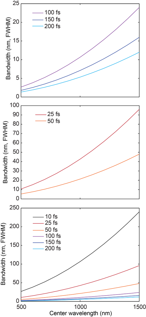
I usually run into pulses that are best described as sech^2. That’s what these graphs are for. I made curves for several different pulse widths (FWHM), and plotted them on different scales for comparison.

Here’s the code to generate the graphs above, which are for sech^2 pulses, and graphs for Gaussian pulses.

%% time-bandwidth product

c= 3*10^8;

pw = [10 25 50 100 150 200];    % pulse width in fs
wl = 500:100:1500;              % wavelength in nm

G_bw_Hz = 0.44./(pw.*10^-15);   % bandwidth in Hz, for Gaussian pulses
S_bw_Hz = 0.32./(pw.*10^-15);   % bandwidth in Hz, for Sech^2 pulses

G_bw_nm = zeros([numel(pw) numel(wl)]);
S_bw_nm = zeros([numel(pw) numel(wl)]);

for n=1:numel(wl)
    w=wl(n).*10^-9;
    G_bw_nm(:,n)=(10^9).*(G_bw_Hz.*w^2)/c;
    S_bw_nm(:,n)=(10^9).*(S_bw_Hz.*w^2)/c;
end

figure
subplot(1,2,1)
plot(wl,S_bw_nm)
subplot(1,2,2)
plot(wl,G_bw_nm)