Snappy looking calcium imaging videos
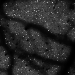
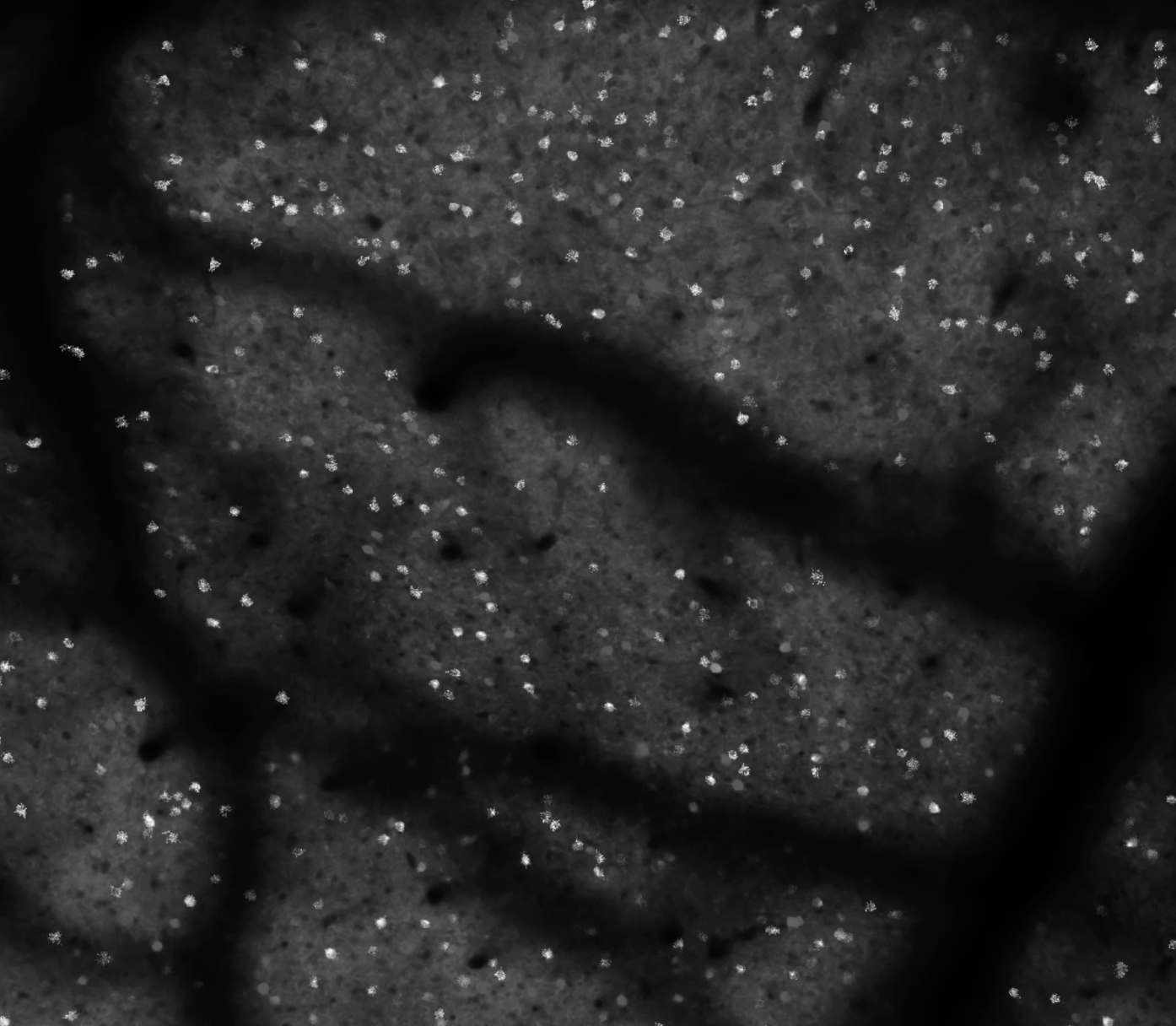
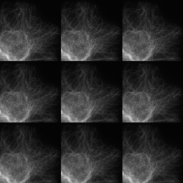
Want to make your calcium imaging videos look better for presentations? Read on. Or just skip to the recipe section below. First, I’ll discuss the motivation a bit.
One of my refrains…
Want to make your calcium imaging videos look better for presentations? Read on. Or just skip to the recipe section below. First, I’ll discuss the motivation a bit.
One of my refrains…
Years ago, Benjamin Judkewitz wanted to try some new techniques out with laser scanning two-photon microscopy. However, the software we were using was rather cumbersome to modify. So he wrote his own software…
One of the most common ways that universities and institution use to evaluate scientists is to solicit letters of recommendation. But who should they ask? Of course former mentors will write letters. To…
This post is from Rob Campbell:
As part of TENSS we have created a set of examples showing how to use DAQmx in MATLAB without the Data Acquisition Toolbox. This…
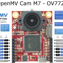
OpenMV is an open source machine vision system. It’s designed to be easy-to-use, with a gentle learning curve. They want this to be the “Arduino of Machine Vision”. The software IDE…
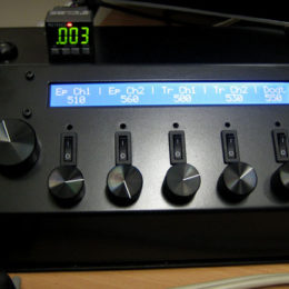
I was cleaning house a bit, and among my old files I found this, which might be worth sharing. Years ago I made a centralized power supply for a custom 2-photon imaging system I built. There…
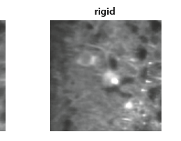
We recently tweeted about a preprint from Eftychios A Pnevmatikakis and Andrea Giovannucci (code). The preprint is on motion correction for calcium imaging data. It is a nice quick read and discusses earlier work…
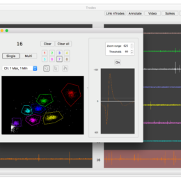
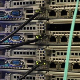
SpikeGadgets makes hardware and software for extracellular array recording.
They make nice looking hardware, both for recording from arrays, and for controlling experiments.
…
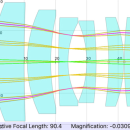
RayLab is an iOS app (iPhone/iPad) for optics analysis. It has some nice features– more than I expected. It’s a nice piece of work! For many practical applications it cannot replace conventional optic design software…
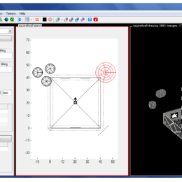
Dmitriy Aronov, while postdocing in David Tank’s lab at Princeton, developed a virtual reality engine that runs in MATLAB called ViRMEn. It’s open and there’s a good amount of documentation. The…
Slack is very useful team coordination software. It’s been such a help in my own lab, that I suspect that given a properly configured Slack account, I could simultaneously run GE, Google, Intel, and…
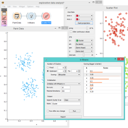
Orange is a user friendly, graphical data mining package built with Python, from the University of Ljubljana. Check it out. They have a good blog for the project…
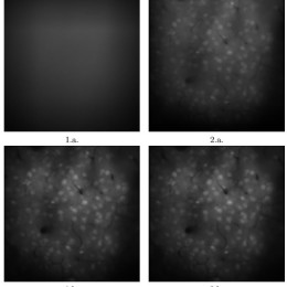
Results are similar to the slow version of TurboReg, but it runs about twice as fast as the fast version of TurboReg.
Here’s the paper.
Here’s the code.
…
Peng Xi (Peking University) shared this resource his lab has developed: software for processing images for structured illumination (a superresolution technique).
Here’s the Github repository.
And here’s the paper…
It’s still early days, but this looks impressively good. Ufora might be one of the easiest-to-try ways to use parallel computing. With just a couple of lines of code, you can run…