
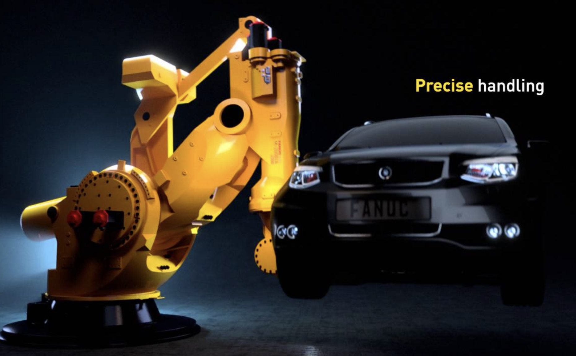
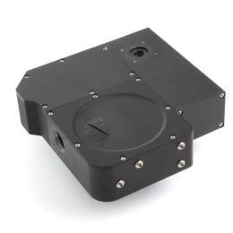
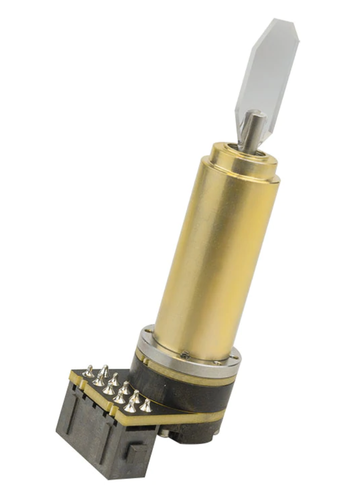
Robot arm with a 2p scope attached
Posted in Hardware
Coming soon to your neuroscience lab.
Thorlabs has worked with the great Jacob Reimer to create a streamlined 2p system that is compact enough to mount on a robotic…
Coming soon to your neuroscience lab.
Thorlabs has worked with the great Jacob Reimer to create a streamlined 2p system that is compact enough to mount on a robotic…
There are some companies that have no real competition. Maybe a product here-and-there in their catalog is subject to market forces, but most of their items have no competing options…
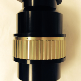
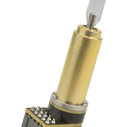
Several people have reached out for guidance on designing and building an objective from scratch, when they have little-to-no background in custom optics. Here are some notes on the topic, in broad strokes, focused on the practicalities.
…
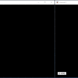
Years ago, Benjamin Judkewitz wanted to try some new techniques out with laser scanning two-photon microscopy. However, the software we were using was rather cumbersome to modify. So he wrote his own software…
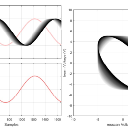
This could be handy for some of you. Resonant scanners are fast, but inflexible. You can’t tell them where to go. They just oscillate at a fixed frequency. All you can do is control…
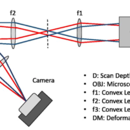
There are lots of ways to quickly change the z-focus plane, including tunable lenses, piezo objective movers, and a coupled objective. What is the best way to change the…
Post by Amanda Foust
Applications are invited for the above post to work with Dr. Amanda Foust (Bioengineering department) and Prof. Pier Luigi Dragotti (Electrical and Electronic Engineering department) on a BBSRC funded…
Frontiers in BioImaging 2018 will take place on Wednesday 27 and Thursday 28 June at the Technology and Innovation Centre, Glasgow. It will focus on the latest developments in applications of…
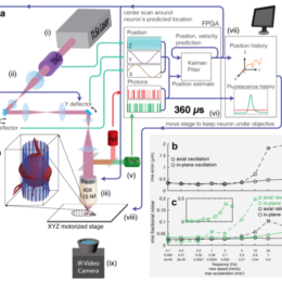
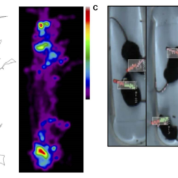
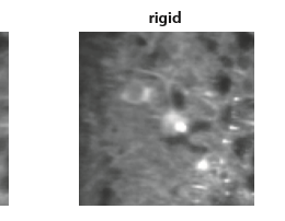
In this work, the authors used fast optical motion tracking and 2p imaging to measure the activity of individual neurons in freely moving animals. No surgery. No optical window. No restraint. And all the…
This post is from Rob Campbell:
As part of TENSS we have created a set of examples showing how to use DAQmx in MATLAB without the Data Acquisition Toolbox. This…
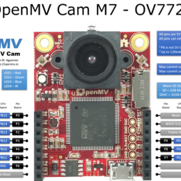
OpenMV is an open source machine vision system. It’s designed to be easy-to-use, with a gentle learning curve. They want this to be the “Arduino of Machine Vision”. The software IDE…
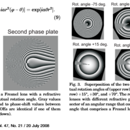
Moiré lenses are cool: two patterned diffractive optical elements are rotated relative to each other to vary the power of the “lens”. Just watch the video (below).
Demonstration of focus-tunable diffractive Moiré-lenses
Stefan Bernet,…
Pixy is an open source computer vision system. Mostafa Nashaat, Robert Sachdev, and colleagues including Matthew Larkum have developed software for use with the Pixy, that can be used to track mouse behavior, including free movement…
We recently tweeted about a preprint from Eftychios A Pnevmatikakis and Andrea Giovannucci (code). The preprint is on motion correction for calcium imaging data. It is a nice quick read and discusses earlier work…

Max Planck Florida is running their imaging course again and there’s still time to apply. They’ve got great faculty including Na Ji, Ryohei Yasuda, Yi Zuo, Chris Xu, Jeff Lichtman, Naomi Kamasawa,…