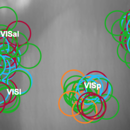
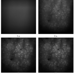
Posts tagged with imaging

December 31, 2011

Optimizing pulse frequency for 2p imaging

The lasers used in multiphoton imaging deliver their photons in pulses. Many commonly used systems pulse at 80 MHz. However, there are good reasons to try different frequencies.

In 2007, Donnert, Eggeling, and Hell published a Nature Methods paper where they used low frequency pulses to get more fluorescence signal out of the preparation. The idea was that many molecules get excited into triplet states that are long-lived. By having a long time between pulses, there is time for the molecules to fall back down into the ground state so that the next pulse will have a large population of molecules available to be excited.

The next year, Ji, Magee, and Betzig published a Nature Methods paper where they used high frequency, low power pulses to get an increase in signal-to-noise ratio with two-photon imaging.

Several people have been confused by these apparently contradictory results. Recently there was a discussion on the Confocal Listserv about this topic, again pointing out the differences between the two papers.

Andrew Ridsdale chimed in with his thoughts (link to post). One of his points is that in different experiments, different factors are limiting the signal.

In Hell’s experiments with low pulse rates, they were imaging cell-free molecules– a very bright signal. Bleaching (triplet-state occupancy) was the limiting factor, rather than damage. Because there weren’t even any cells around to be damaged, other than E. coli cells in the last figure. So allowing for relaxation time and maximum occupancy of the ground state gave the best results. All of the relevant processes were governed by 2p excitation and thus were second order.

In the Ji, Magee, and Betzig experiments, the signals were very dim (not unusually dim for slice experiments, but dimmer than the preparations used by Donnert et al.) and the limiting factor was damage to the preparation. Andrew’s point seems to be that in this case, the signal is coming from second order processes and the damage is from higher order processes, maybe even as high as 5th order, though they estimate it to be on average about 2.4 order. So in this case, it’s best to use pulses that are just barely effective for 2p excitation and completely ineffective for higher order processes (damage), and then blast the prep with as many pulses as possible. Since the likelihood of a 2p event is already low, bleaching isn’t as much of a factor.

(btw, Brain Windows did a very nice post on the Ji and Donnert papers)

0 comments

November 30, 2011

An Arch-based voltage sensor

The newest voltage sensor is from Adam Cohen’s lab and based on a microbial rhodopsin, a class of light sensitive proteins already being put to use in optogenetics.

In this case, they’ve take Archaerhodopsin 3 (a related protein to Arch, which has been used to hyperpolarize neurons and silence activity) and removed it’s ion fluxing ability. But since it still senses voltage and light, its optical characteristics change with voltage.

How does it compare with existing voltage sensors? It has a relatively large change in fluorescence over a physiological voltage range (about 50%), but it’s very slow (41 ms onset). They can nicely see APs in single sweeps in cultured cells. In slices and in vivo, the signals will be smaller. One of the best voltage imaging schemes around, DiO+DPA, has a similar fluorescence change and is way faster (<1 ms). Note that signals from Arch(D95N) in culture (top picture below) don’t look massively better than DiO+DPA in slice (bottom picture below). Hopefully Arch(D95N)’s signals will still be usable in slices and in vivo.

Arch(D95N) in culture

DiO+DPA in slice

But of course, having a genetically targettable construct is a huge advantage. So a fairer comparison would be to other voltage sensing proteins. In that case, Arch(D95N)’s fluorescence change is excellent, but its slow speed is a handicap and makes that big fluorescence change less useful. Perhaps the biggest problem with Arch(D95N) is that it’s dim. The quantum yield is 9e-4 and an EMCCD was required for these experiments. For comparison, many GFP based proteins have quantum yields over 5e-1. It’s extiction coefficient is decent– it absorbs light– it’s just really unlikely to emit a fluorescence photon.

Maybe the protein engineers will follow up and make a brighter and faster version, the authors themselves report that they’re actively working on speed. For what it’s worth, the native protein (with it’s fluxing capability intact) is much faster, so there’s hope on that front.

Knopfel has taken perhaps the most rigorous and deliberate approach to voltage sensing protein design. The first big problem is that the sensor has to be at the membrane, so unlike calcium sensors, the signal-generating ROI is pretty small. The second big problem is that the sensor adds an unnatural capacitance to the membrane, so when expression levels increase to improve S:N, the capacitance also increases and messes up excitability. They have a nice analysis in this paper.

Nevertheless, there’s a lot to do with voltage sensors and I don’t think people have really started to fully explore what they’re capable of. These systems don’t need to be perfect, there is a huge amount of physiology to explore even using the existing voltage sensors.

0 comments

November 27, 2011

Thorlabs’ B-scope

Thorlabs’ scope pieces and kits have been mentioned in these pages before. At SfN, they had their new B-scope on display. This is like the Sutter MOM and the UCLA scope, in that the microscope rotates in one plane in addition to x-y-z movement. A few differences with the Thorlabs scope:

1. The objective rotates around the focal plane, and the rotation is motorized.
With the Sutter/UCLA style scopes, the objective rotates about an axis along the scan path, so the focus point changes a ton when rotating. The rotation can really only be changed before there is a prep on there, because the objective swings a big arc whenever the rotation changes and it ends up pointing at a completely different point in space.

By contrast, the Thorlabs scope is set up to rotate about an axis that is in the plane of focus. So you can be looking at a cell and then, while imaging, rotate the scope (since it’s motorized) and still keep looking at the same thing, just from a different angle.

This is why they have the crazy periscope you can see to the right in the photo below.

I remember seeing a scope with this same feature (rotation around an axis in the image plane) at a conference at least 2 years ago. I think it was a group based out of Switzerland. Can anyone fill in the details for me?

2. No conventional scanners, just the Thorlabs conventional scanners.
This might not be true for long. Thorlabs has their own conventional scanners, but they’re not as fast as Cambridge Technologies (CTI) scanners. This is probably why they opted to put their resonant scanners in the system.

I’m guessing that they’ll help out buyers if they want to fit the scope with a set of conventional scanners from CTI. I say this because Thorlabs told more than one person at SfN that they would help them fit the Thorlabs resonant scanner kit to their Sutter MOM scope. This was news to Sutter.

0 comments

November 12, 2011

TIRF teaching materials

Next time you’re explaining TIRF to someone, start off by showing them this piece of artwork. (Arndt von Scheidt, source)

3 comments

November 11, 2011

Building a 2p scope, 2011 edition

What’s new this year?

The original post on building a 2p scope still gets a lot of hits. Let’s revisit the topic.

Scientifica

Scientifica has been working hard on developing a kit for multiphoton imaging. It’s all based off of their minimalist, yet versatile SliceScope platform.

I’ve had the opportunity to check out their collection module and it’s really well done. The components are available for individual purchase, so if you just want to buy part of it and tack it onto something else you’ve got, they offer that flexibility. Since they sell a wide range of electrophysiology products, they can offer customized package deals to suit your needs.

The collection module shown above is a nice tight package with the PMTs, filter cube, and preamps all integrated. They really like the R9880U series. I can see why: they’re very small, with an 8 mm diameter active area, and are constructed such that incident light can approach from a wide angle. However, they are bialkali and the QE at 520nm is less than 30%. They have a GaAsP version in the works.

Their platform can be configured for slices (below, left) or in vivo (below, right).

Thorlabs

Thorlabs has made some improvements in their own software for their 2p kit, and Vijay Iyer’s ScanImage 4 will interface with the resonant scanners. I think this is an interesting starting place for custom rigs. Thorlabs has add-ons like deformable mirrors that you can purchase at a later time. There’s no conventional galvo scanning option, and since resonant galvos are not good for arbitrary line scanning, you’re pretty much locked into (fast) raster scanning. If that’s not an issue, it’s a good option. And I’m guessing they’ll have a conventional galvo scanning option at some point– they do actually sell them, all they have to do is integrate it into the software. Neither their software nor ScanImage 4 supports regular galvo scanning at this time, but at least the latter intends to add that functionality.

Till Photonics

Till Photonics has a couple of systems on offer too. First up is the 2p version of their iMIC platform. These octagonal monoliths look like they should be launched into space.

Till Photonics’ modules are popular, particularly their Yanus scan head. The heart of it is a set of Cambridge Technologies 6210s, but they have them packaged up nicely in top quality optics and an easy-to-implement module. They have modelled the nonlinearities and can squeeze a bit more scan speed out of the mirrors if you use their systems.

Next up from Till is their Intravital 2p that came out this spring.

It boasts a fairly large scan field (about 15.5 mm to a side in the focus plane, divide by your objective’s magnification to get the field of view) and a voice-coil driven z-axis with 7.5 mm of travel.

By the way, Till Photonics runs Colibri, an open source, LabVIEW-based laser scanning microscope software package. It runs off of the NI PCI-6110 board that most people use. It’s modular, uses 4 MHz sampling, and has support for cameras, motor controllers, and beam control. So you don’t have to have a Till system to try out the software. The author, Christian Seebacher, has some interesting information about the software on his website.

I’m sure there’ll be more new stuff at SfN this year… let me know if you see anything interesting.

0 comments

November 1, 2011

Thorlabs’ SM2 fits Nikon lenses

Fun fact for the day: ThorLabs’ SM2 lens tube standard screws right onto the front end of Nikon’s SLR lenses. Other manufacturers probably use the same threading, I just haven’t tried them.

I don’t know if this is by design or not, but it makes coupling 35mm SLR lenses into optical setups fairly straightforward. I’m using it for a tandem lens macroscope. In the picture above I used ThorLabs part SM3A2. BTW, they also sell some F-mount adapters for connecting to the other side of the lens.

1 comments

October 17, 2011

Photon counting, addendum

Let me add some clarification to the hybrid PMT post.

The actual signal that comes off of a PMT in response to a photon is a pulse of current. The amplitude of this pulse can vary wildly, and the variation is referred to as multiplicative noise. For that reason, photon counting schemes typically use a simple threshold-crossing to trigger counts, which often mostly solves multiplicative noise. You’re smart, so I know you’re already wondering what happens when two pulses occur very close to each other in time. This is called “pile up” and it’s a problem. There are different ways to deal with it, but since single pulses can be so variable, it’s difficult to deal with it effectively. I also want to note that even for dim images, events WILL come close enough together SOMETIMES. And for bright images, it happens quite often, and this precludes quantitative imaging.

Hybrid PMTs address this by having a huge gain at the first stage which essentially decreases the noise (by a factor of sqrt(n)) so that the photon-evoked pulses are less variable. They can also be designed to make the pulses briefer. Brief pulses = less pileup, and more regular pulses means that more sophisticated schemes can be used to accurately count photons. All in all, this results in more quantitative imaging. Of course, this is most relevant for bright images.

Alright, back to watching Plaxico Burress not catching passes.

1 comments

October 16, 2011

Photon counting with Hybrid PMTs

Hybrid PMTs have made their way into fluorescence microscopy and are competing with GaAsP PMTs. (Well, actually, Hamamatsu makes both types, so it’s not really competition in that sense.) These devices have a huge gain at the first stage, which results in lower multiplicative noise. But does it matter? And is it worth the trade off (e.g., some hybrids have smaller detector areas compared to GaAsP PMTs)?

This was the topic of a few recent (and long) posts on the Confocal Listserv. If you’re into this sort of thing, they make a great read.
James Pawley’s post
George McNamara’s post
Wolfgang Staroske’s post

The take-home message is that hybrid PMTs will keep you in a more linear range for bright images.

Some people have noticed higher S:N when they upgraded to hybrid PMTs. But without knowing what their old PMTs were, it’s hard to say that they can offer better images than a top-of-the-line, non-hybrid GaAsP PMT. Your milage may vary and all that. In any case, for dim images, there’s probably not much of an advantage. But for bright images, Hybrid PMTs can offer more quantitative images.

This all is most relevant in photon counting mode. Hybrid PMTs give less variable signals in response to single photons because of the high gain in the first stage.

(an application note on hybrid PMTs from Becker-Hinckl)

1 comments

September 24, 2011

GECOs – New proteins for calcium imaging

Post by Christian Wilms

Call me old-fashioned, but I’m a big fan of small organic calcium indicators (e.g., Oregon Green BAPTA 1). Yes, genetically encoded calcium indicators (GECIs) have many advantages: targeting to specific cell populations, subcellular targeting, etc. But for quantitative, high SNR work, OGB-1 & Co. (ideally not as an AM-ester) is where it’s at.

There are several reasons for this: GECIs have fairly small signal amplitudes (commonly on the level of under 10-fold fluorescence increase from calcium free to calcium bound). They are slow, with on- and off-rates several orders of magnitude slower than BAPTA-based indicators. They are only available in two overlapping hues (green or blue/yellow) limiting the combinability with other indicators and dyes. Finally, the link between [Ca2+] and GECI fluorescence is very non-linear, making quantification difficult.

Not that there hasn’t been any progress over the past decade: the fluorescence increase on calcium binding has steadily increased over the years, the introduction of troponin-C in place of calmodulin as a binding domain has caused a mild increase in kinetics and there have been some preliminary presentations of spectrally shifted GECIs. But all in all, a big jump ahead has not happened yet.

That was the situation until two weeks ago, when Rob Campbell’s lab published an exciting report: Using a bacteria-based high throughput screen, they scanned tens of thousands of randomly generated mutations of GCaMP3. Using this approach they developed a series of GECOs (for Genetically Encoded Calcium indicators for Optical imaging). Among this series is a green fluorescing indicator (G-GECO) with a 26-fold intensity change on binding calcium, a red indicator (R-GECO) with a 16-fold change and a blue indicator (you guessed it: B-GECO) with a more humble 4-fold increase. In addition they developed an emission ratiometric indicator (GEM-GECO) with a flabbergasting 110-fold ratio change as well as an excitation ratiometric indicator (GEX-GECO) with a 26-fold change in ratio.

While the kinetics are still in the same range as those of previous GECIs, the combination of different spectral variants and large dynamic range does address to major limitations of earlier GECIs. Finally, to make a good thing better, the authors will be making all the GECIs open to public access by depositing them at addgene.org.

0 comments

July 17, 2011

2pLSM: When will scientists stop making their own?

In the early days of patch clamp electrophysiology, everyone made their own patch clamp amplifiers because there were none commercially available. I was lucky enough to be educated by scientists of such lineage, and in one of my classes, as an exercise, we built a simple patch clamp amplifier with series resistance compensation.

Even after patch clamp amplifiers became commercialized, there were still a few aficionados who insisted on their own designs. But very quickly, companies started building so much technology into the amplifiers, that the amps surpassed what an aficionado could practically engineer in their own labs. Although expensive, the amps were affordable and offered a great deal of functionality.

Perhaps 2-photon laser scanning microscopes (2pLSMs) are approaching a similar turning point. With the expiration of the patent on 2pLSM and the flood of commercial interests in the market, including open source designs like the Janelia Farm scope pictured above (link), we are starting to see much more technology being built into these scopes.

Features such as high speed scanning and wavefront shaping are becoming commonplace. Although both of these can easily be implemented on custom built scopes, the pace of “featurization” of scopes is picking up. Perhaps in five to ten years, no one will be building their own scopes anymore because companies are selling such high tech scopes at very competitive prices.

This website is about open solutions for science, but this is primarily motivated by efficiency, i.e., not reinventing the wheel. We’ll keep covering custom 2pLSM information, for now, but only as long as it is practical. We do not anticipate covering how to build a custom patch clamp amplifier, but it could happen.

Optimizing pulse frequency for 2p imaging