Postdoc job: Zebrafish, Natural scenes, Thiele lab, Toronto
Posted in Uncategorized
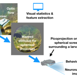
The Thiele Lab at the University of Toronto is recruiting a Postdoc for the Fall to work with an HFSP team (UC Berkeley, Univ of Maryland, and Univ of Tübingen) that is investigating population…